A sweep with figures

This tutorial runs an external-aerodynamics case at two angles of attack in one job: one mesh, two freestream conditions, an early stop at each, and a rendered figure set per point. It assumes you finished your first job.

You need a case whose 0/U has a freestreamVelocity patch, a forceCoeffs function object named coeffs, and runTimeModifiable true. Cases written by TerraHawk’s cfd_case.py have all three. Stage it on the server first, its STL files included, as Stage a case without a shell shows.

1. Submit the sweep.

   submit_sweep({
     "case_name": "flight-a6.7-b0-coarse",
     "points": [{"alpha": 6.7}, {"alpha": 8}],
     "stop": "watcher"
   })

   The steps it returns show the shape of the job: the mesh chain once, then for each point a setPoint step that rewrites the freestream on the decomposed fields, a solver step, and a render step, then a strip that puts every point’s view A side by side.

2. Follow the mesh. While snappyHexMesh runs, the summary line names its phase and cell count:

   snappyHexMesh (4/9) snapping 2.86M cells

   If you pass expected_cells, a final count more than 3% above it raises the cell_count_leak check after meshing, which usually means the surface leaked.

3. Watch the first point converge. Use wait_for with until: "converged". The watcher computes the spread of Cd, Cl and CmPitch over the trailing 200 iterations, and once all three are steady it lowers endTime so the point ends early. The summary line then ends with converged, ends at 620 (the new end), and the event solver.converged records the iteration and the rule.

4. Let the second point run. It starts from the first point’s converged fields, so it settles in a fraction of the iterations. job_status lists both points with their window means.

5. Read the coefficients. job_coeffs with point: 1 returns mean, standard deviation, min, max and spread for every column over the trailing window of the alpha 8 point. job_forces splits the forces by patch group.

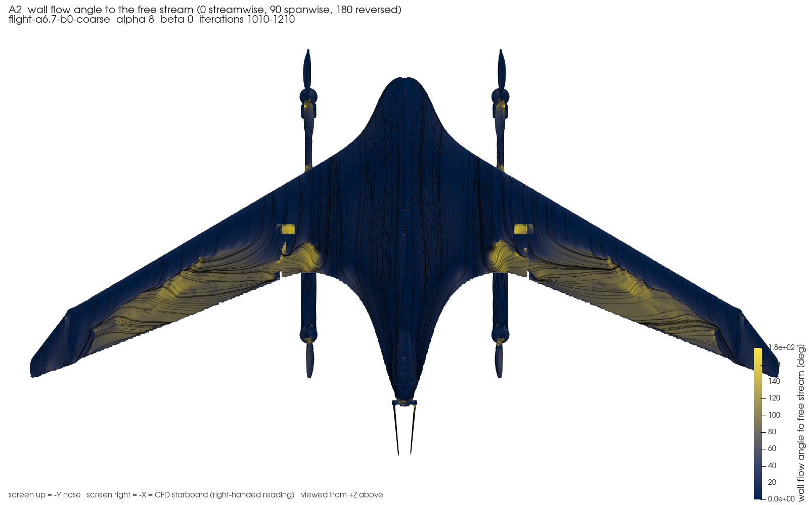
6. Look at the figures. job_figures lists one set per point. Ask for figures/p1/A.png and Claude reads it through the job:// resource.

View A2 for the alpha 8 point: the angle between the wall flow and the free stream. The yellow band over the aft outer wing is flow at 120 to 140 degrees, running spanwise and partly forward. It is the same region view A shows as near-zero streamwise friction.

Why one mesh

Two separate meshings of the same geometry differ by about one percent in drag. That is larger than many of the effects worth measuring between neighbouring angles. A sweep removes it, because every point shares the identical mesh.

What you did

You ran a two-point polar on one mesh, stopped each point on a convergence rule rather than a guessed iteration count, and got figures without opening a desktop. Add points to a finished sweep shows how to fill in a gap later without meshing again.